Appendix 1: Discussion Supplementary Materials
The following Supporting Information is available for the discussion:
Fig. 17. Principal component analyses of leaf functional traits for Symphonia and Eschweilera clade Parvifolia species.
Fig. 18. Growth trajectories of Symphonia and Eschweilera clade Parvifolia species.
Fig. 19. Site frequency spectra for Symphonia species.
Fig. 20. Phylogeny for Symphonia species.
Fig. 21. Variance partitioning of leaf functional traits in Symphonia species.
Fig. 22. Functioncal traits and individual growth potential for Symphonia species.
Fig. 23. Leaf thickness variation with precipitation for Symphonia species.
Fig. 24. Effect of sampling on the estimate of the species mean trait value within Symphonia species.
Fig. 25. Variance partitioning for neighbourhood crowding index and individual growth potential in Eschweilera clade Parvifolia species.
Fig. 26. Local basal area distribution prior to basal area loss in Paracou.
Simulator S1. C++ code for the one-dimension eco-evolutionary simulator.
Simulator S2. R code for the two-dimensions eco-evolutionary simulator.
Fig. 27. Species variation in growth trajectories of Symphonia and Eschweilera clade Parvifolia species.
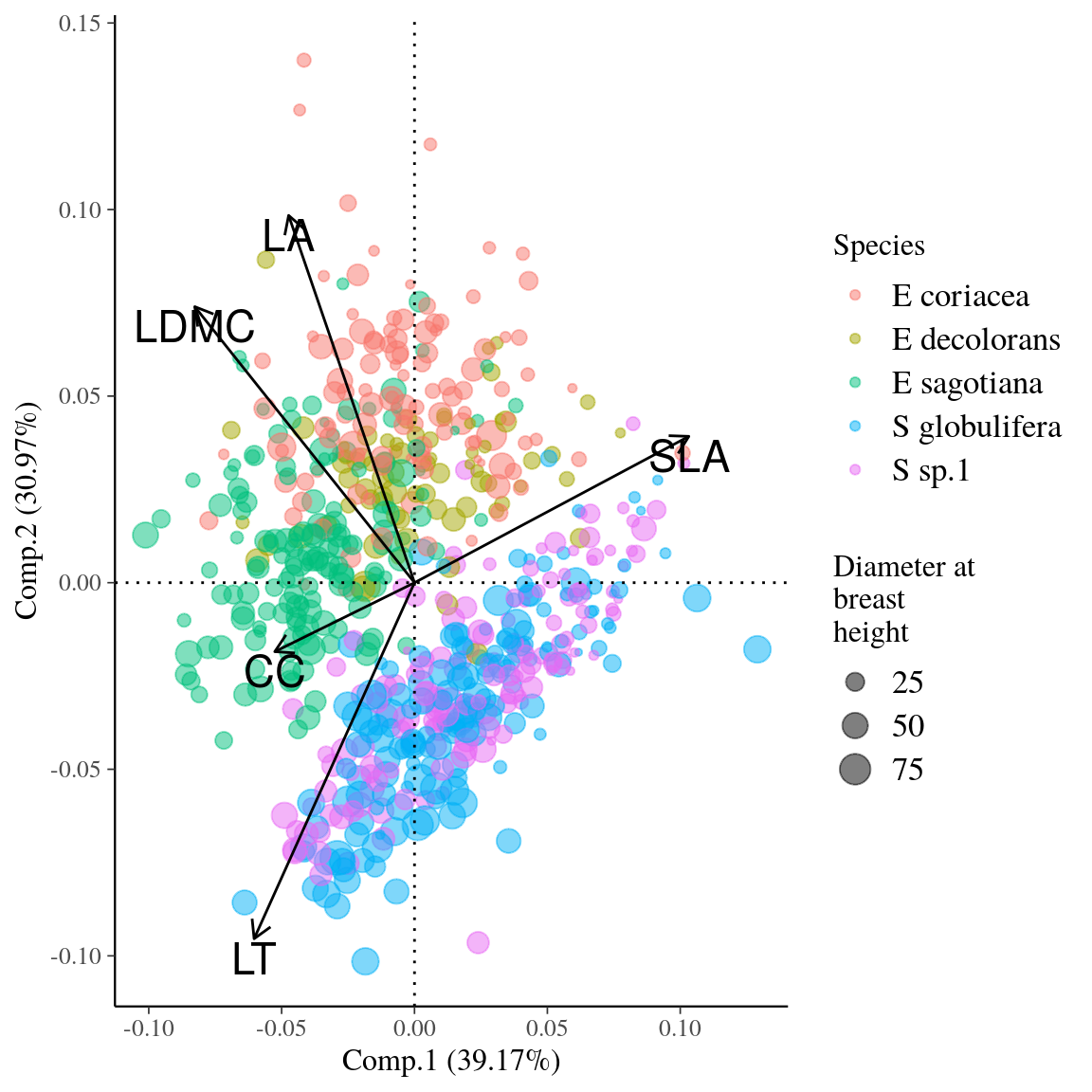
Figure 17: Principal component analyses of leaf functional traits for Symphonia and Eschweilera clade Parvifolia species. Dot colors indicate the species, whereas dot sizes indicate diameter at breast height.
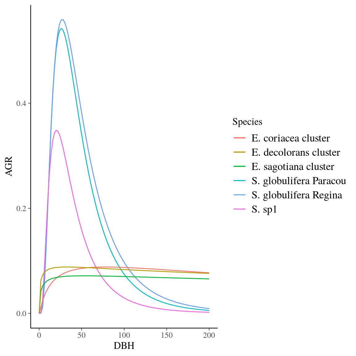
Figure 18: Growth trajectories of Symphonia and Eschweilera clade Parvifolia species.
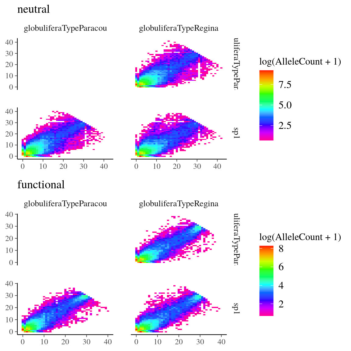
Figure 19: Pairwise site frequency spectra for Symphonia species. We used the genome-transcriptome alignments built for the design of probes sets to classify called SNPs into (i) anonymous SNPs, i.e. neutral (on scaffolds matching no transcripts), and (iii) genic SNPs, i.e. functional (within an exon).
![Phylogeny for *Symphonia* species. Drift-based phylogeny of *Symphonia* and *Pentadesma* populations with `treemix` [@Pickrell2012]. Subfigure **A** present the log-likelihood of the phylogeny topology depending on the number of allowed migration events per SNP type, suggesting 1 migration event to better represent the phylogeny topology than none. Others subfigures represent the phylogeny for anonymous (**B**), genic (**C**) and putatively-hitchhiker (**D**) SNPs. The red arrow represents the most likely migration event. Population are named by their localities, including *Symphonia* species only or *Symphonia* and *Pentadesma* species in Africa. At the exception of the three Paracou populations: *S. sp1*, *S. globulifera type Paracou* and *S. globulifera type Regina* respectivelly named Ssp1, SgParacou and SgRegina.](thesis_files/figure-html/A1symphoniaphylogeny-1.png)
Figure 20: Phylogeny for Symphonia species. Drift-based phylogeny of Symphonia and Pentadesma populations with treemix (Pickrell and Pritchard 2012). Subfigure A present the log-likelihood of the phylogeny topology depending on the number of allowed migration events per SNP type, suggesting 1 migration event to better represent the phylogeny topology than none. Others subfigures represent the phylogeny for anonymous (B), genic (C) and putatively-hitchhiker (D) SNPs. The red arrow represents the most likely migration event. Population are named by their localities, including Symphonia species only or Symphonia and Pentadesma species in Africa. At the exception of the three Paracou populations: S. sp1, S. globulifera type Paracou and S. globulifera type Regina respectivelly named Ssp1, SgParacou and SgRegina.
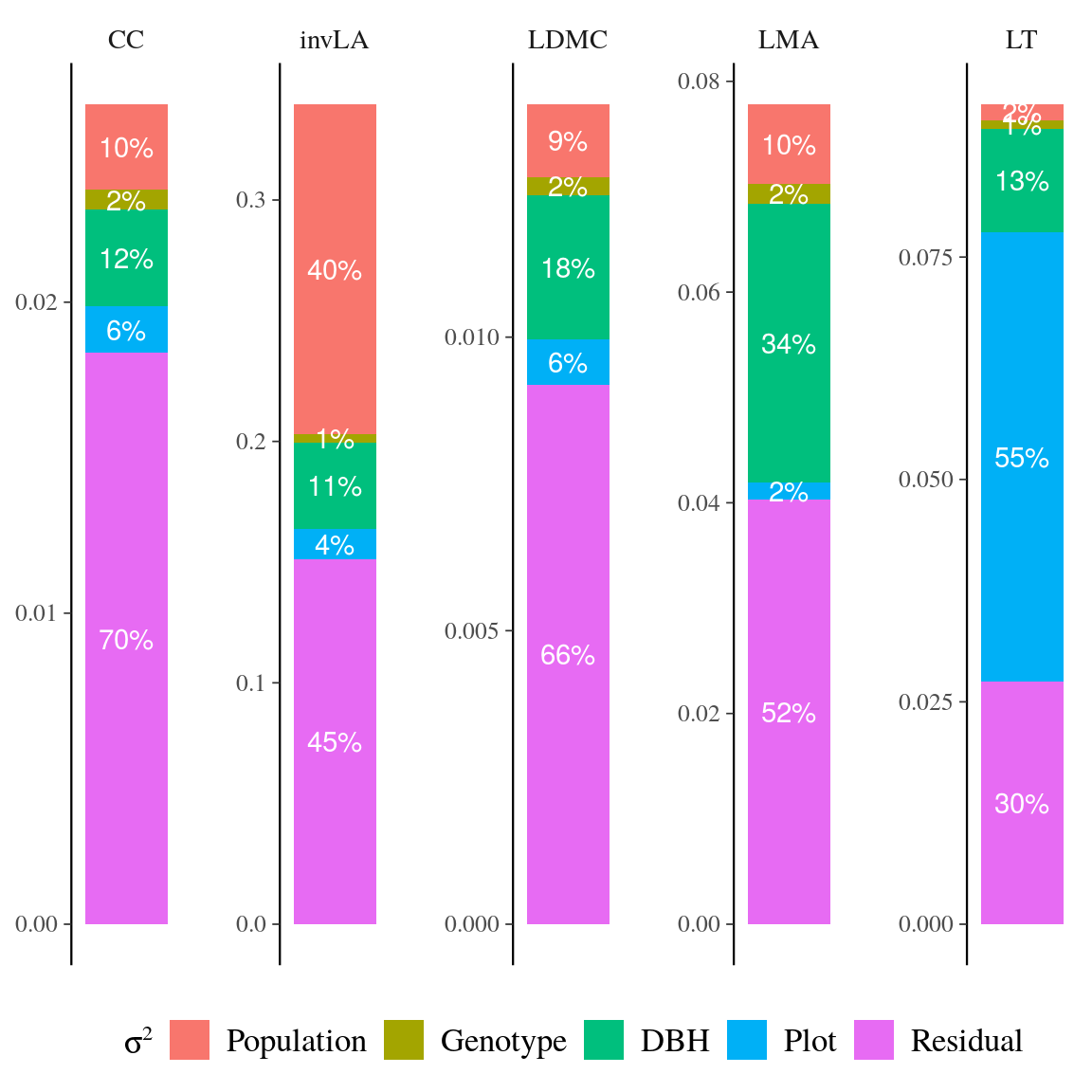
Figure 21: Variance partitioning of leaf functional traits in Symphonia species. …
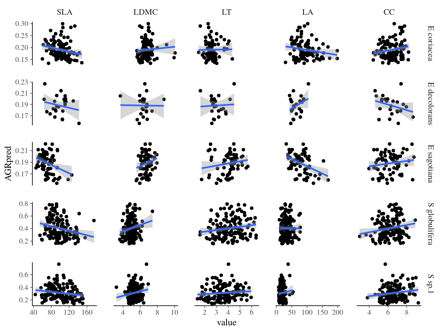
Figure 22: Functioncal traits and individual growth potential for species. Individual growth predicted in 2015 against sampled trait value in 2015.
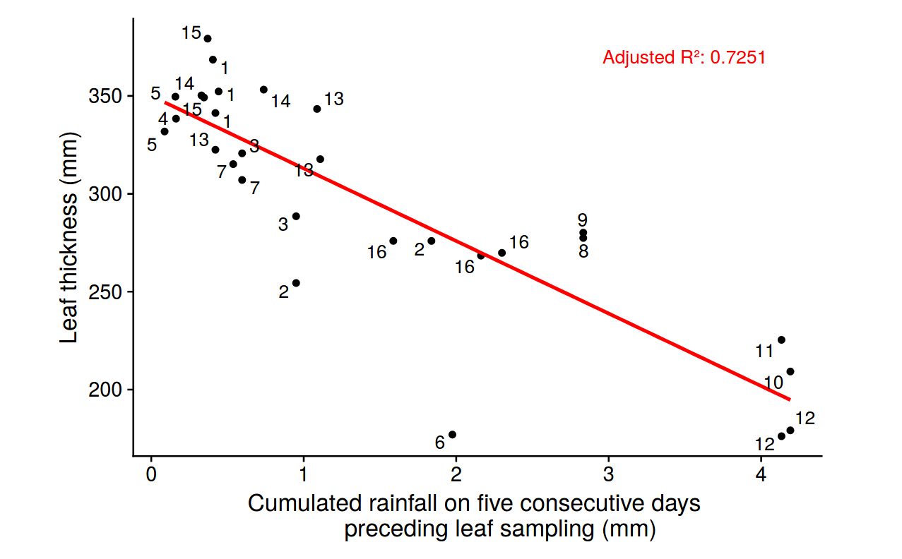
Figure 23: Leaf thickness variation with precipitation for species. Leaf thickness in milimeters against cumulated rainfall on five consecutive days preceeding leaf sampling in milimeters.
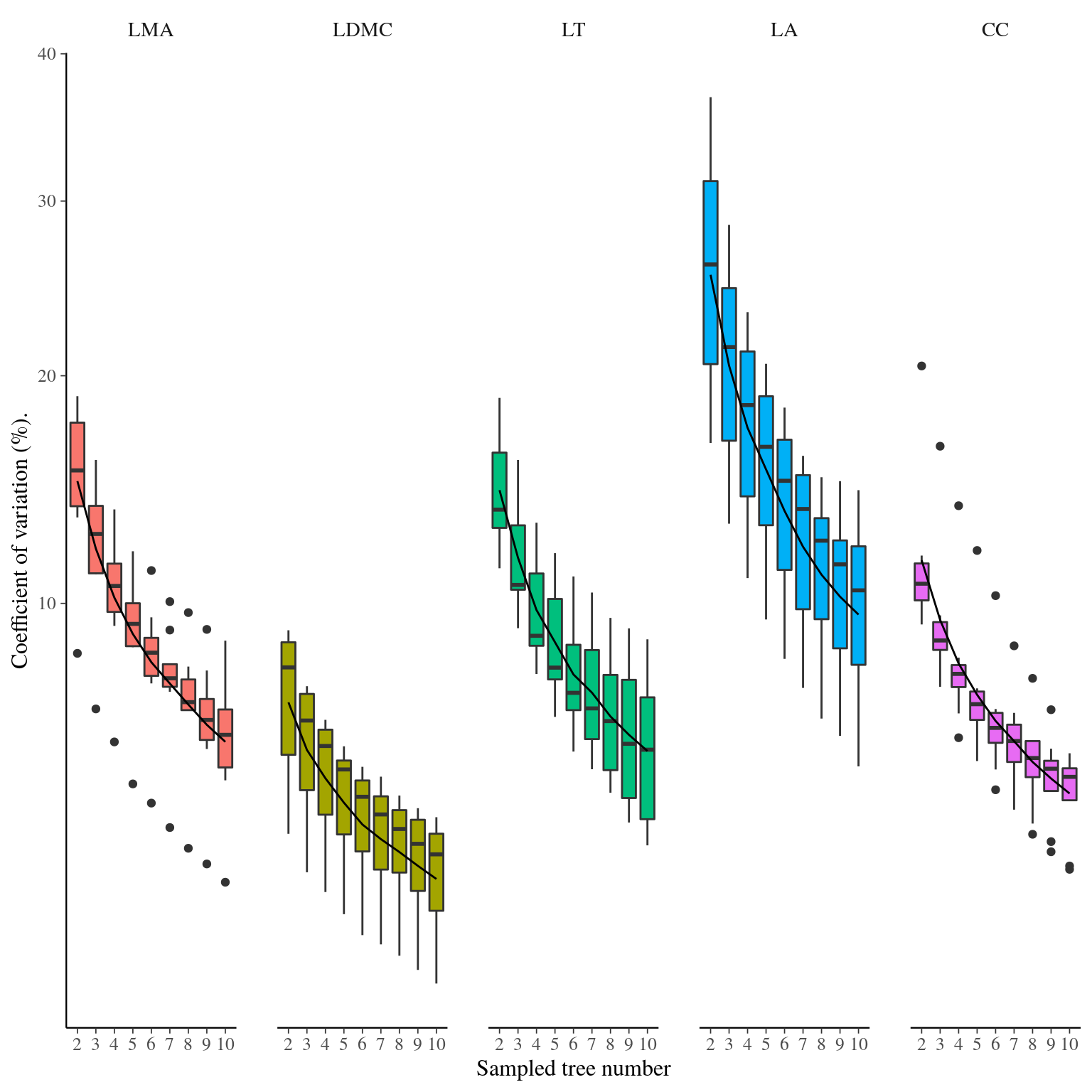
Figure 24: Effect of sampling on the estimate of the species mean trait value within species. Coefficient of variation of mean estimation depending on the number of individuals sampled of DBH>30 cm.
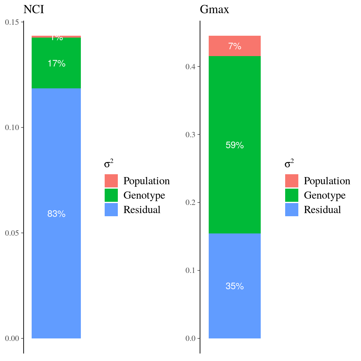
Figure 25: Variance partitioning for neighbourhood crowding index (NCI) and individual growth potential (Gmax) in Eschweilera clade Parvifolia species. Variance partitioning for neighbourhood crowding index (NCI), an indirect measurement of access to light, and individual maximum growth potential (Gmax). Variation of each variable has been partitioned into between-species (red), between-genotype (green), and residual (blue) variation.
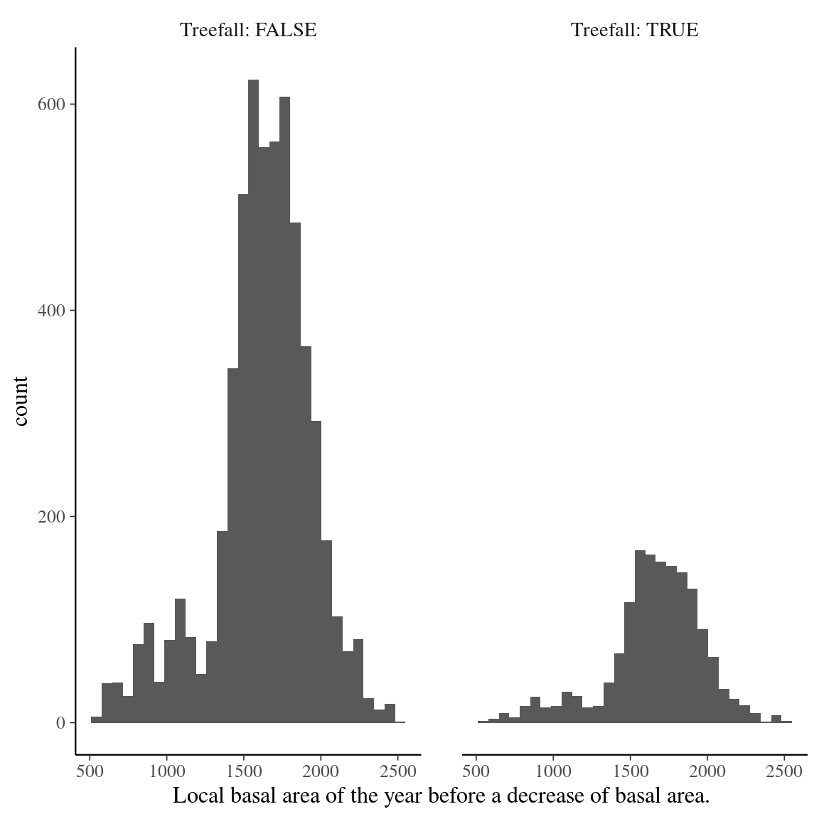
Figure 26: Local basal area distribution prior to basal area loss, i.e. the successional stage of the forest patch before a treefall occurs. Treefall are defined is a loss of basal area superior to 10.
Simulator S2: R code for the one-dimension eco-evolutionary simulator.
#include <Rcpp.h>
using namespace Rcpp;

// [[Rcpp::export]]
NumericVector build_gradient(
    double gradientlim,
    int length
){
  double step = gradientlim*2/(length-1) ;
  NumericVector gradient(length) ;
  gradient[0] = - gradientlim ;
  for (int i = 1; i < length; i++)
    gradient[i] = gradient[i-1] + step ;
  return gradient ;
}

// [[Rcpp::export]]
List simulator1D_cpp(
    int  Nind = 50,
    int Ngen = 50,
    double muG = 0,
    double sigmaG = 1,
    double muE = 0,
    double sigmaE = 1,
    double Elim = 10,
    int seedlings = 4,
    int dispersal = 1,
    bool viability_deterministic = true
) {
  NumericMatrix A(Ngen, Nind) ;
  NumericMatrix Z(Ngen, Nind) ;
  NumericVector E = build_gradient(Elim, Nind) ;
  NumericMatrix Aoffsprings(Nind, seedlings) ;
  NumericMatrix Zoffsprings(Nind, seedlings) ;
  NumericVector Ap(2*dispersal+1) ;
  NumericVector w(seedlings) ;
  IntegerVector seeds(seedlings) ;
  int imin , imax, winner ;
  double muS ;
  A.row(0) = rnorm(Nind, muG, sigmaG) ;
  Z.row(0) = rnorm(Nind, muE, sigmaE) ;
  for(int s = 0; s < seedlings; s++)
    seeds(s) = s ;
  for (int g = 1; g < Ngen; g++){
    for (int i = 0; i < Nind; i++){
      imin = 0 ;
      imax = Nind ;
      if(i-dispersal > 0){
        imin = i-dispersal ;
      }
      if(i+dispersal+1 < Nind){
        imax = i+dispersal+1 ;
      }
      NumericVector Ap(imax-imin) ;
      for(int p = 0; p < imax-imin; p++) Ap(p) = A(g-1,imin+p) ;
      for (int s = 0; s < seedlings; s++){
        Aoffsprings(i,s) = rnorm(1, mean(sample(Ap, 2)), sigmaG/2)[0] ;
        Zoffsprings(i,s) = Aoffsprings(i,s) + rnorm(1, muE, sigmaE)[0] ;
      }
      if(viability_deterministic){
        winner = which_min(sqrt(pow(Zoffsprings(i,_)-E(i), 2))) ;
      } else {
        w = 1/sqrt(pow(Zoffsprings(i,_)-E(i), 2)) ;
        winner = sample(seeds, 1, true, w)[0] ;
      }
      A(g,i) = Aoffsprings(i,winner) ;
      Z(g,i) =  Zoffsprings(i,winner) ;
    }
  }
  List sim = List::create(Named("A") = A,
                          Named("Z") = Z,
                          Named("E") = E) ;
  return sim;
}
Simulator S2: R code for the two-dimensions eco-evolutionary simulator.
simulator2D <- function(
    grid = 20, # size
    Ngen = 50,
    muG = 0, # genetics
    sigmaG = 1,
    muE = 0, # environment
    sigmaE = 1,
    Elim = 5,
    seedlings = 4, # reproduction
    dispersal = 1,
    viability_deterministic = T
){
    A <- array(dim = c(grid, grid, Ngen)) # objects
    Z <- array(dim = c(grid, grid, Ngen))
    A[,,1] <- array(rnorm(grid*grid, muG, sigmaG), dim = c(grid,grid))
    Z[,,1] <- A[,,1] + array(rnorm(grid*grid, muE, sigmaE),
                             dim = c(grid,grid))
    E <- seq(-Elim, Elim, length.out = grid) %*%
      t(seq(-Elim, Elim, length.out = grid))
    for(g in 2:Ngen){ # iterations
      Aoffsprings <- array(
        as.vector(
          sapply(1:grid, function(i)
            sapply(1:grid, function(j)
              sapply(1:seedlings, function(s)
                rnorm(1,
                      sample(A[max(1,i-dispersal):min(i+dispersal,grid),
                               max(1,j-dispersal):min(j+dispersal,grid),
                               g-1], 2),
                      sigmaG/2)
              )
            )
          )
        ), dim = c(grid, grid, seedlings))
        Zoffsprings <- Aoffsprings +
          array(rnorm(grid*grid*seedlings, muE, sigmaE),
                dim = c(grid,grid,seedlings))
        if(viability_deterministic){
            survivors <- array(apply(
              apply(Zoffsprings, 3,
                    function(x) as.array(sqrt((x - E)^2),
                                         dim = c(grid,grid))), 1, which.min),
              dim = c(grid,grid))
        } else {
          survivors <- array(
            apply(1/apply(Zoffsprings, 3,
                          function(x) as.array(sqrt((x - E)^2),
                                               dim = c(grid,grid))), 1,
                  function(w)
                    sample.int(seedlings, 1, replace = T, prob = w)),
            dim = c(grid,grid))
        }
        A[,,g] <- Aoffsprings[cbind(rep(1:grid, grid), rep(1:grid, each = grid),
                                    as.vector(survivors))]
        Z[,,g] <- Zoffsprings[cbind(rep(1:grid, grid), rep(1:grid, each = grid),
                                    as.vector(survivors))]

    }
    return(lapply(list("breeding value (a)" = A, "trait value (z)" = Z),
                  function(M)
        reshape2::melt(M) %>%
          dplyr::rename(X = Var1, Y = Var2, generation = Var3)) %>%
        bind_rows(.id = "var") %>%
          left_join(reshape2::melt(E) %>%
                      dplyr::rename(X = Var1, Y = Var2, environment = value),
                    by = c("X", "Y")) %>%
          mutate(individual = paste0("X",X,"Y",Y)))
}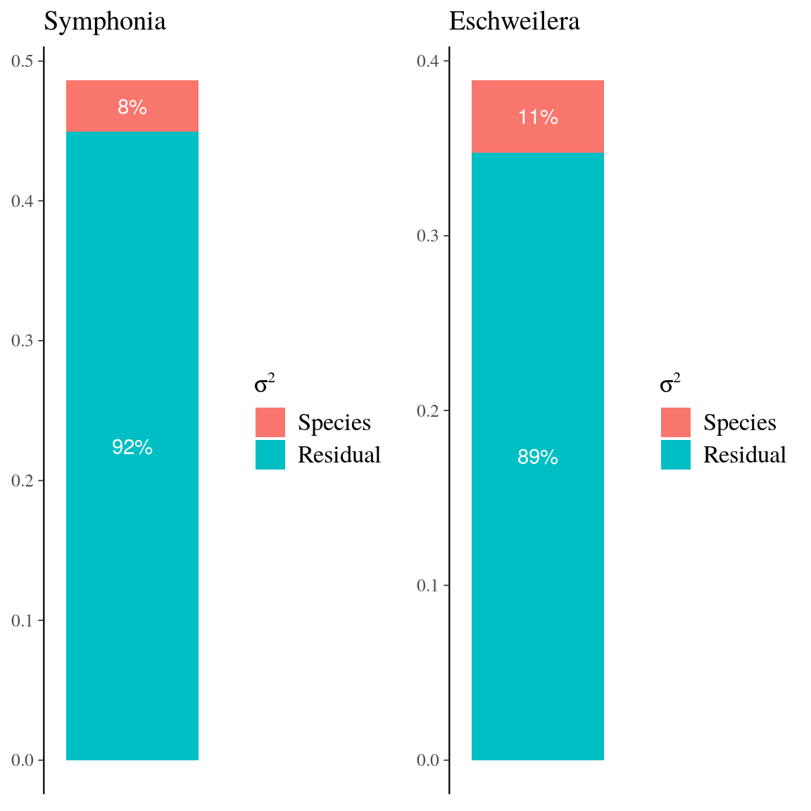
Figure 27: Species variation in growth trajectories of Symphonia and Eschweilera clade Parvifolia species.
References
Pickrell, J. K. and Pritchard, J. K. 2012. Inference of Population Splits and Mixtures from Genome-Wide Allele Frequency Data. - PLoS Genetics in press.