Appendix 4: Chapter 3 Supplementary Materials

Article title: Topography drives microgeographic adaptations among closely-related species of two tropical tree species complexes

Authors: Sylvain Schmitt, Niklas Tysklind, Bruno Hérault, Myriam Heuertz

The following Supporting Information is available for this article:

Method S1. Design of the probes set for Symphonia.

Method S2. Design of the probes set for Eschweilera.

Model S1. Stan code for the animal model

Tab. 10. Eschweilera botanical species and genetic clusters

Fig. 36. Target selection for the capture experiment of Symphonia

Fig. 37. Target selection for the capture experiment of Eschweilera

Fig. 38. SNP abundance per library for Eschweilera

Fig. 39. Library abundance per SNP for Eschweilera

Fig. 40. Outgroup detection for Eschweilera

Fig. 41. Cross-validation for Symphonia population structure

Fig. 42. Symphonia population structure using admixture

Fig. 43. Symphonia population structure using hybrid index

Fig. 44. Outlier SNPs among Symphonia species

Method S1: Design of the probes set for Symphonia.

For Symphonia globulifera, the genomic and transcriptomic resources used for the design were comprised of a published low-coverage draft genome from Africa (Olsson et al. 2017), an unpublished draft genome from French Guiana [Scotti et al., in prep], an unpublished transcriptome from 20 juveniles from French Guiana [Tysklind et al., in prep], and reduced-representation genomic sequence reads of individuals from French Guiana [Torroba-Balmori et al., unpublished]. We aligned genomic reads on the two genome drafts with bwa (Li and Durbin 2009). We kept scaffolds from the two genome drafts with a length superior to 1 kbp and at least one matching alignment with a read with a single match on the genome, and merged the two filtered genome drafts with quickmerge (Chakraborty et al. 2016). We aligned transcripts on the new filtered genome draft with BLAT (Kent 2002) and selected 533 scaffolds without transcript-match, i.e. anonymous scaffolds. We masked repetitive regions with RepeatMasker (Smit et al. 2015) and selected 533 1-kbp anonymous loci within the 533 previous scaffolds.

Similarly, we filtered transcripts from the 20 juveniles of Symphonia globulifera from French Guiana [Tysklind et al., in prep] based on SNP quality, type and frequency. We further detected open reading frames (ORFs) using transdecoder (Haas et al. 2013), and selected transcripts with non-overlapping ORFs including a start codon. We kept ORFs with an alignment on scaffolds from the aforementioned genome draft for Symphonia using BLAT (Kent 2002), and masked repetitive regions with RepeatMasker (Smit et al. 2015). We selected 1,150 genic loci of 500-bp to 1-kbp, from 100 bp before the start to a maximum of 900 bp after the end of the ORFs, resulting in 1-Mbp genomic loci that included a coding region.

Method S2: Design of the probes set for Eschweilera.

For Eschweilera, the genomic and transcriptomic resources used for the design were comprised of transcriptomes from Eschweilera sagotiana and Eschweilera coriacea (Vargas et al. 2019), and unpublished reduced representation genomic reads (M. Heuertz pers. com.). We mapped reciprocally E. coriacea and E. sagotiana transcriptomes using BLAT (Kent 2002), and in reciprocal best matches, we kept a single transcript to avoid paralogs and have robust targets among species. We further detected open reading frames (ORFs) using transdecoder (Haas et al. 2013), and selected transcripts with non-overlapping ORFs including a start codon. We selected 1,530 transcriptomic loci of 500-bp to 1-kbp, from 100 bp before the start to a maximum of 900 bp after the end of the ORFs, resulting in 0.83-Mbp of transcriptomic loci. To build anonymous targets, we built a de novo assembly of ddRAD-seq genomic data using ipyrad (Eaton and Overcast 2020), mapped consensus sequences on transcripts using BLAT (Kent 2002), and kept consensus sequences with no match on transcripts. We masked repetitive regions with RepeatMasker (Smit et al. 2015) and selected 2.2k anonymous loci resulting in a length 0.52-Mbp.

Model S1: Stan code for the bayesian inference of the animal model.

data {
  int<lower=0>  N ; // # of individuals
  int<lower=0>  P ; // # of populations
  real y[N] ; // phenotype
  int<lower=1, upper=P> population[N] ; // populations
  cov_matrix[N] K ; // kinship covariance matrix
}
transformed data{
  matrix[N, N] A = cholesky_decompose(K) ; // cholesky-decomposed kinship
  real Vy = variance(log(y)) ;
}
parameters {
  vector<lower=0>[P] mu ; // intercept
  vector[N] epsilon ; // genotypic noise
  real<lower=0, upper=sqrt(Vy)> sigma ; // genetic variance
}
transformed parameters {
  real<lower=0> Vp = variance(log(mu[population])) ; // population variance
  real Vr = square(sigma) ;
  real Vg = Vy - Vp - Vr ;
  vector[N] alog = sqrt(Vg)*A*epsilon ;
}
model {
  y ~ lognormal(log(mu[population]) + alog, sigma) ;
  epsilon ~ std_normal() ;
  mu ~ lognormal(0, 1) ;
  sigma ~ normal(0, 1) ;
}

Table 10: Confusion matrix (percentage) between genetic cluster and botanical identification for clade .

Species	E. coriacea cluster	E. decolorans cluster	E. sagotiana cluster
E. coriacea	65	8	13
E. decolorans	15	77	7
E. sagotiana	20	16	80

Figure 36: Scheme of target selection for the capture experiment of as described in the manuscript.

Figure 37: Scheme of target selection for the capture experiment of clade as described in the manuscript.

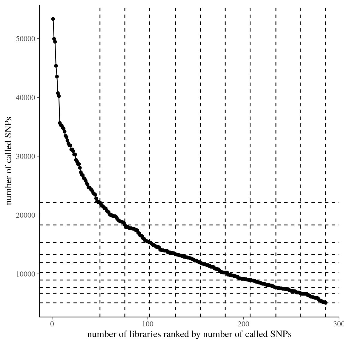
Figure 38: SNP abundance per library rank for raw data of clade . Dashed lines represent tested filters.

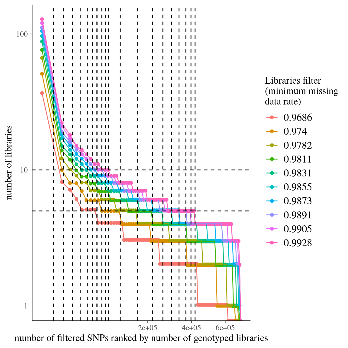
Figure 39: Library abundance per SNP rank for library-filtered data of clade . Dashed lines represent tested filters.

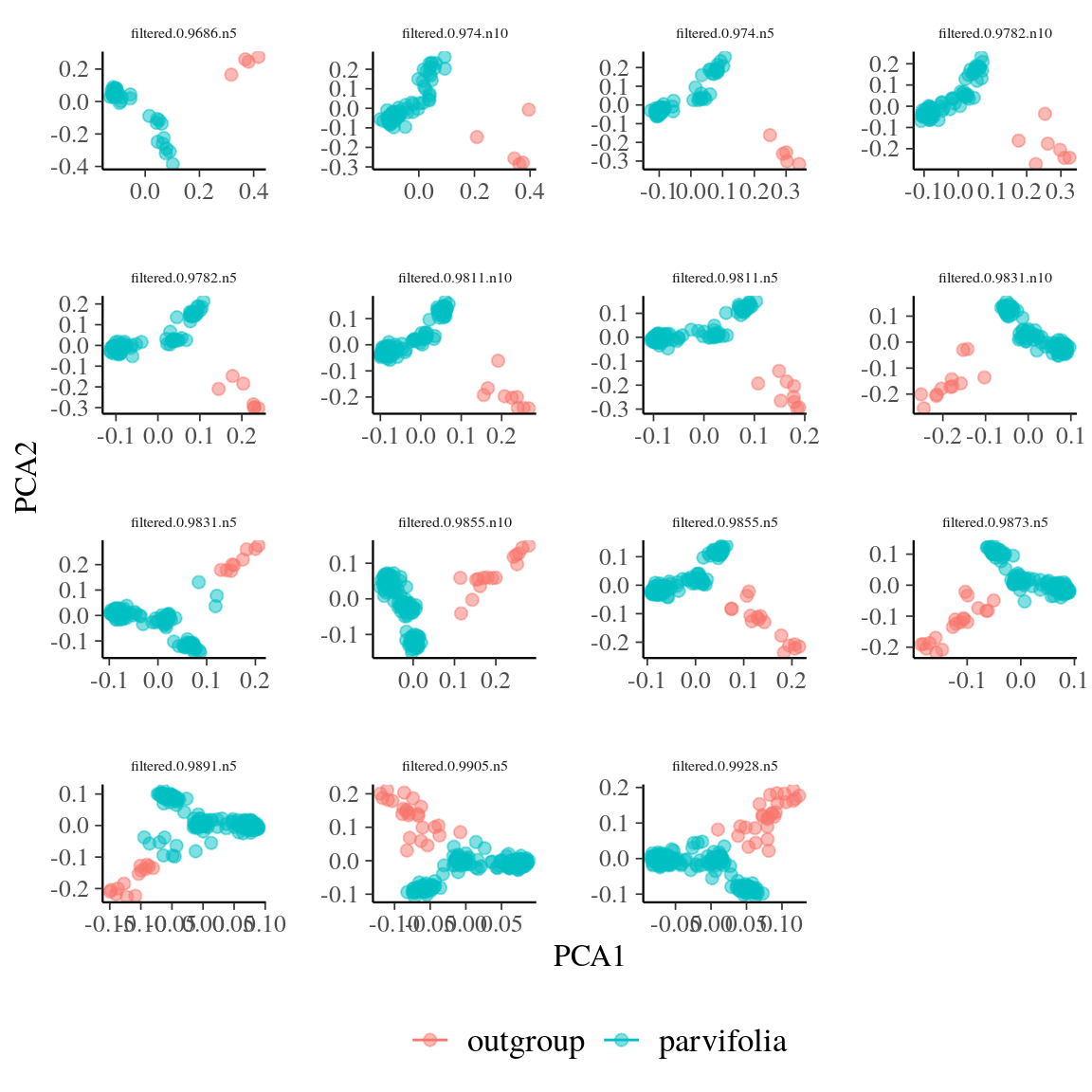
Figure 40: Outgroup detection with individual clustering in the genomic principal component analysis (gPCA) in two groups using K-means for every filter.

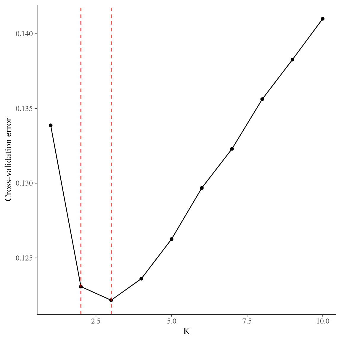
Figure 41: Cross-validation for the clustering of individuals using admixture. Y axis indicates cross-validation mean error, suggesting that K = 2 or K = 3 gene pools represent the best solution for genetic structure in in Paracou.

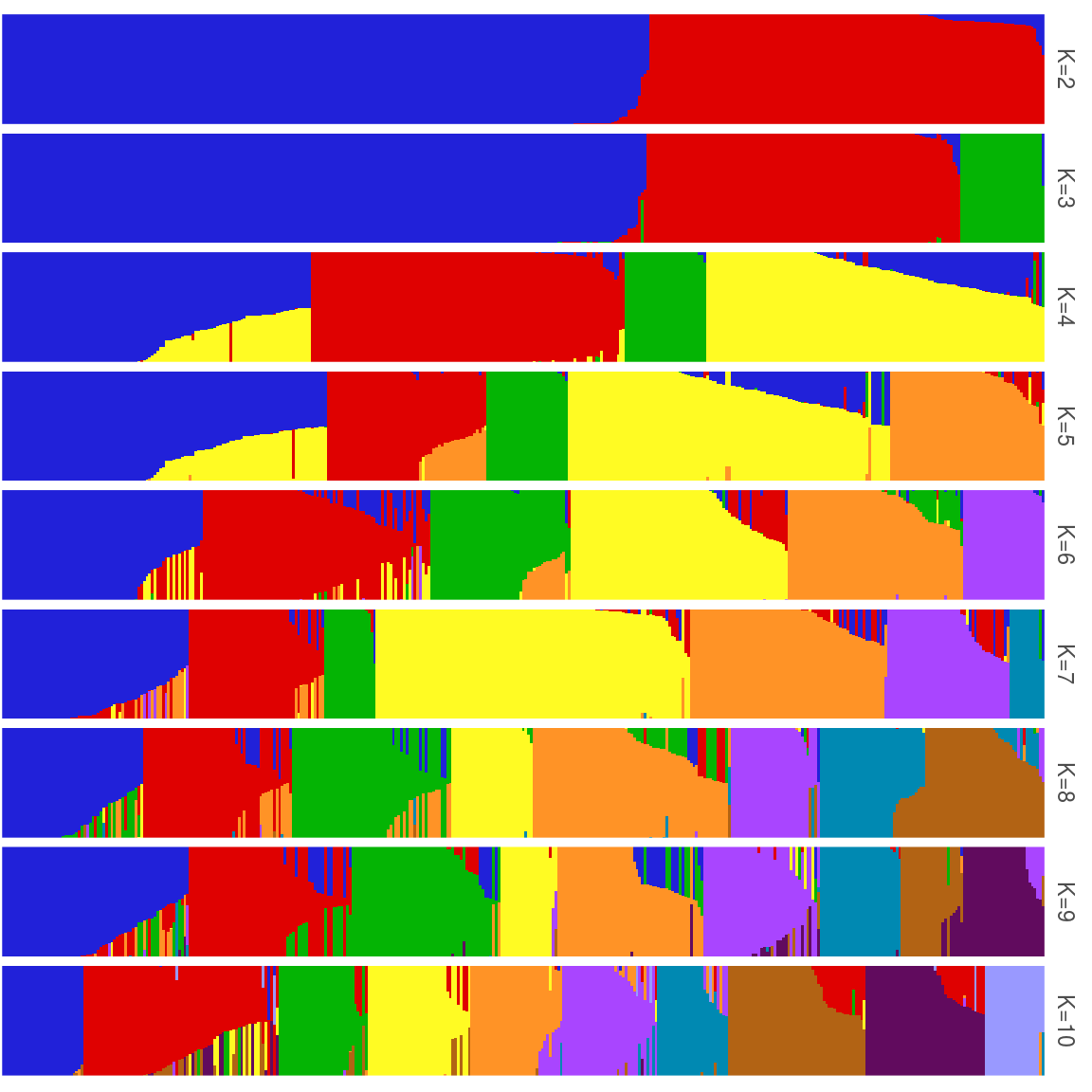
Figure 42: Population structure of individuals from K=2 to K=10 using admixture.

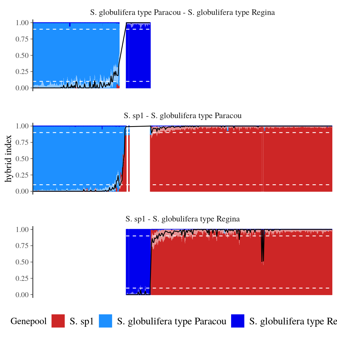
Figure 43: Genotypinc constitution of using hybrid index. Admixture coefficients (black line) are given with 90% confidence interval (light shade). Admixture coefficients of 10 and 90% are indicated by white stippled lines.

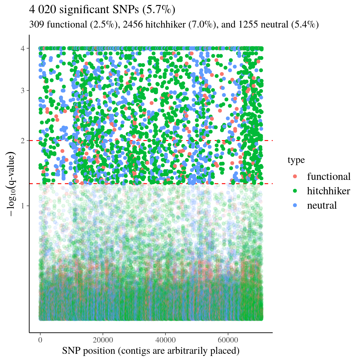
Figure 44: High-differentiation outlier SNPs for individuals detected with bayescan. We used the genome-transcriptome alignments built for the design of probes sets (Method S1) to classify called SNPs into (i) anonymous SNPs (on scaffolds matching no transcripts), (ii) putatively-hitchhiker SNPs (close to a transcript or within an intron), and (iii) genic SNPs (within an exon).

References

Chakraborty, M. et al. 2016. Contiguous and accurate de novo assembly of metazoan genomes with modest long read coverage. - Nucleic Acids Research 44: 1–12.

Eaton, D. A. and Overcast, I. 2020. ipyrad: Interactive assembly and analysis of RADseq datasets. - Bioinformatics (Oxford, England) 36: 2592–2594.

Haas, B. J. et al. 2013. De novo transcript sequence recostruction from RNA-Seq: reference generation and analysis with Trinity.

Kent, W. J. 2002. BLAT—The BLAST-Like Alignment Tool. - Genome Research 12: 656–664.

Li, H. and Durbin, R. 2009. Fast and accurate short read alignment with Burrows-Wheeler transform. - Bioinformatics 25: 1754–1760.

Olsson, S. et al. 2017. Development of genomic tools in a widespread tropical tree, Symphonia globulifera L.f.: a new low-coverage draft genome, SNP and SSR markers. - Molecular Ecology Resources 17: 614–630.

Smit, A. et al. 2015. RepeatMasker Open-4.0.: <http://www.repeatmasker.org>.

Vargas, O. M. et al. 2019. Target sequence capture in the Brazil nut family (Lecythidaceae): Marker selection and in silico capture from genome skimming data. - Molecular Phylogenetics and Evolution 135: 98–104.