Appendix 2: Chapter 1 Supplementary Materials

Article title: Topography shapes the local coexistence of tree species within species complexes of Neotropical forests

Authors: Sylvain Schmitt, Niklas Tysklind, Géraldine Derroire, Myriam Heuertz, Bruno Hérault

The following Supporting Information is available for this article:

Fig. 28. Correlation of abiotic topographic variables and neighbor crowding indexes.

Tab. 6. Model tested for species complex distribution.

Fig. 29. Habitat suitability of single taxa model for every model form.

Tab. 7. Model parameters for each complex with scaled descriptors.

Tab. 8. Model parameters for each complex with scaled descriptors.

Model S1. Stan code for the inference of species complex presencer.

Model S2. Stan code for the inference of species joint-presence.

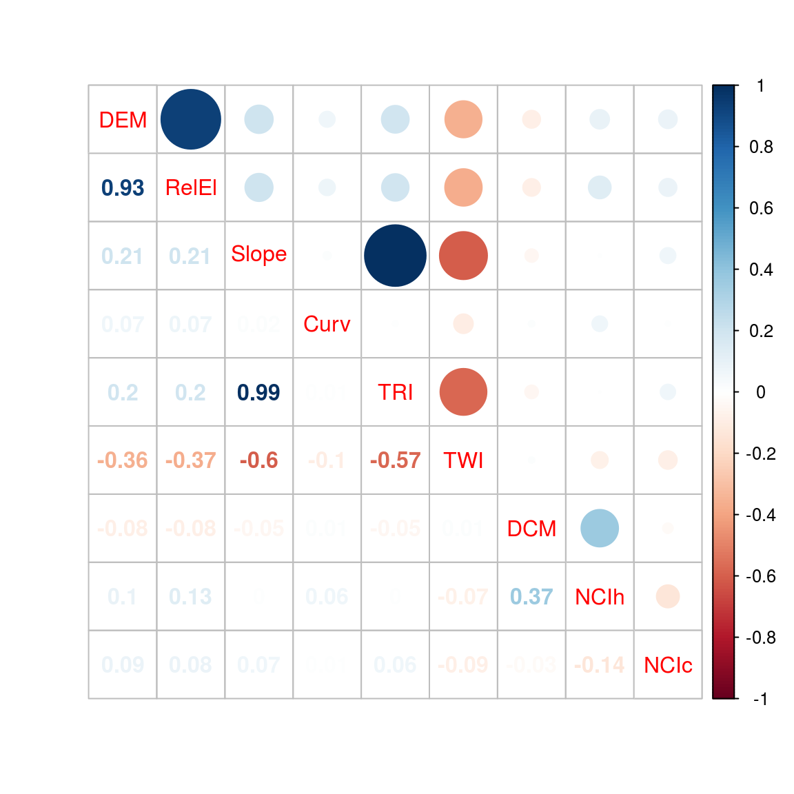
Figure 28: Correlation of abiotic topographic variables and neighbor crowding indexes (NCI). All variables, relative elevation (RelEl), slope, curvature (Curv), aspect, topographic ruggedness index (TRI), and topographic wetness index (TWI) are derived from the digital elevation model (DEM) obtained through LiDAR campaign in 2015, the digital canopy model (DCM) has been obtained in the same campaign, and neighbor crowding index (NCI) of heterospecific (NCIh) or conspecific (NCIc) are derived from Paracou census campaign of 2015.

Table 6: Model tested for species complex distribution.

Name	Formula
$B_0$	$Presence\sim Bernoulli\left(logi{t}^{-1}\right({\alpha }_0\left)\right)$
$B_{\alpha }$	$Presence\sim Bernoulli\left(logi{t}^{-1}\right({\alpha }_0+\alpha \ast Environment\left)\right)$
$B_{\alpha ,{\alpha }_2}$	$Presence\sim Bernoulli\left(logi{t}^{-1}\right({\alpha }_0+\alpha \ast Environment+{\alpha }_2\ast Environmen{t}^2\left)\right)$
$B_{\alpha ,\beta }$	$Presence\sim Bernoulli\left(logi{t}^{-1}\right({\alpha }_0+\alpha \ast Environment+Environmen{t}^{\beta }\left)\right)$
$B_{\alpha ,\beta }2$	$Presence\sim Bernoulli\left(logi{t}^{-1}\right({\alpha }_0+\alpha \ast (Environment+Environmen{t}^{\beta })\left)\right)$
$B_{\alpha ,\beta }3$	$Presence\sim Bernoulli\left(logi{t}^{-1}\right({\alpha }_0+Environmen{t}^{\alpha }+Environmen{t}^{\beta }\left)\right)$

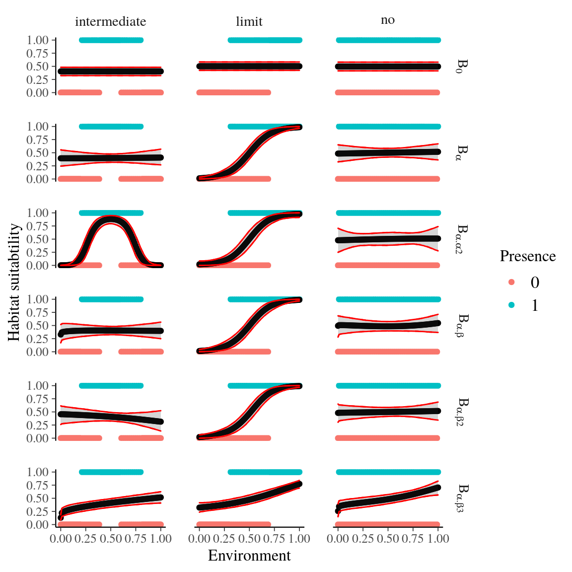
Figure 29: Habitat suitability of single taxa model for every model form (see Supplementary Material Tab. 6) and three theoretical species distribution cases. Three species distribution cases have been simulated: (i) the environmental variable has no effect, (ii) the niche optimum is an intermediate value of the environmental variable range, and (iii) the niche optimum is a limit of the environmental variable range. Blue and red dots represent simulated presences and absences respectively, whereas the black line represents the fitted corresponding model with its credibility interval in grey. The model B,2 shows the best behavior with the three distribution cases.

Table 7: Model parameters for each complex with scaled descriptors.

complex	$\alpha$	${\beta }_{NCI}$	${\beta }_{TWI}$	${\gamma }_{NCI}$	${\gamma }_{TWI}$
Iryanthera	-3.338	-1.414	1.054	0.547	-0.237
Licania	-1.488	-0.716	0.056	-0.017	-0.208
Parvifolia	-1.403	-0.840	0.207	-0.254	-0.193
Symphonia	-2.423	-1.296	-0.110	-0.255	0.106
Talisia	-2.006	-1.699	-0.340	-1.263	0.017

Table 8: Model parameters for each complex with scaled descriptors.

SpeciesLong	$\alpha$	${\beta }_{NCI}$	${\beta }_{TWI}$	${\gamma }_{NCI}$	${\gamma }_{TWI}$
E coriacea	0.954	0.278	1.186	-0.236	-0.142
E decolorans	-0.041	0.244	0.051	0.574	-0.723
E grandiflora_form2	-0.455	-0.520	0.028	-0.557	-0.109
E pedicellata	-0.631	-0.576	-0.033	-0.520	0.145
E sagotiana	1.411	1.444	-1.875	1.299	0.430
E wachenheimii	-1.135	-0.846	0.709	-0.510	0.264
I hostmannii	0.133	-0.228	0.285	-0.538	0.396
I sagotiana	-0.125	0.225	-0.231	0.512	-0.377
L alba	3.459	0.643	-0.048	-2.108	0.362
L canescens	-0.036	0.296	-1.087	0.622	0.462
L laxiflora	-0.234	-0.274	0.086	-0.258	-0.665
L membranacea	-0.164	0.142	1.286	0.487	-0.250
L micrantha	-0.626	-0.003	0.362	0.570	-0.056
L ovalifolia	-0.839	-0.134	0.313	0.512	0.021
L parvifructa	-0.553	-0.651	-0.023	-0.787	-0.362
L sprucei	-0.966	-0.024	-0.910	0.950	0.472
S globulifera	-0.551	-0.754	0.905	-0.937	0.299
S sp.1	0.546	0.716	-0.850	0.986	-0.324
T hexaphylla	0.062	0.213	-0.564	0.417	0.204
T praealta	0.056	-0.101	0.074	-0.230	0.101
T simaboides	-0.155	-0.185	0.477	-0.120	-0.267

Model S1: Stan code for the inference of species complex presence

functions {
  real scale(vector x) {
    return sqrt(sum(x .* x)/(num_elements(x) - 1)) ;
  }
}
data {
  int<lower=1> N ;                // # of individuals
  int<lower=1> K ;                // # of environmental descriptors
  int<lower=0, upper=1> Y[N] ;    // individuals presence or absence (0-1)
  matrix[N,K] X ;                 // environmental descriptors
  int<lower=1> N_pred ;
  matrix[N_pred,K] X_pred ;            
}
transformed data {
  matrix[N,K] X_std ;
  matrix[N_pred,K] X_pred_std ;
  for(k in 1:K) {
    X_std[,k] = X[,k] / scale(X[,k]) ;  
    X_pred_std[,k] = X_pred[,k] / scale(X[,k]) ;  
  }
}
parameters {
  real alpha ;       // intercept
  vector[K] beta ;   // sigmoidal slope
  vector[K] gamma ;  // quadratic form
}
model {
  alpha ~ normal(0, 1) ;
  beta ~ normal(0, 1) ;
  gamma ~ normal(0, 1) ;
  Y ~ bernoulli_logit(alpha + X_std * beta + (X_std .* X_std) * gamma) ;
}
generated quantities {
  vector[N_pred] Y_pred ;
  Y_pred = inv_logit(alpha + X_pred_std * beta + (X_pred_std .* X_pred_std) * gamma) ;
}

Model S2: Stan code for the inference of species joint-presence

functions {
  real dirichlet_multinomial_lpmf(int[] y, vector alpha) {
    real alpha_plus = sum(alpha);
    return lgamma(alpha_plus) + sum(lgamma(alpha + to_vector(y)))
                - lgamma(alpha_plus+sum(y)) - sum(lgamma(alpha));
  }
  real scale(vector x) {
    return sqrt(sum(x .* x)/(num_elements(x) - 1)) ;
  }
}
data {
  int<lower = 1> N  ;       // # of individuals
  int<lower = 1> S  ;       // # of species
  int<lower = 1> K  ;       // # of environmental descriptors
  int<lower = 0, upper=1> Y[N, S]  ; // individuals presence or absence for each species
  matrix[N,K] X ;           // environmental descriptors
  int<lower=0> N_pred ;
  matrix[N_pred,K] X_pred ;
}
transformed data {
  matrix[N,K] X_std ;
  matrix[N_pred,K] X_pred_std ;
  for(k in 1:K) {
    X_std[,k] = X[,k] / scale(X[,k]) ;  
    X_pred_std[,k] = X_pred[,k] / scale(X[,k]) ;  
  }
}
parameters {
  vector[S] alpha ; // intercept
  matrix[S,K] beta ; // sigmoidal slope
  matrix[S,K] gamma ; // quadratic form
}
model {
  alpha ~ normal(0,1) ;  
  for(k in 1:K){
    beta[,k] ~ normal(0,1) ;
    gamma[,k] ~ normal(0,1) ;
  }
  for (n in 1:N)
    Y[n] ~ dirichlet_multinomial(softmax(alpha + beta*to_vector(X_std[n,]) 
                                 + gamma*to_vector(X_std[n,] .* X_std[n,])))  ; 
                                 // likelihood
}
generated quantities {
  matrix[N_pred,S] Y_pred ;
  for(n in 1:N_pred)
    Y_pred[n,] = to_row_vector(softmax(alpha + beta*to_vector(X_pred_std[n,]) 
                               + gamma*to_vector(X_pred_std[n,] .* X_pred_std[n,]))) ;
}